Using masked array with Hi-C map

Large Hi-C map data contains missing values. During analysis, sometimes we need to ignore these values. numpy.ma module can be used to perform mathematical operations after masking these missing values.

See also

Module numpy.ma

---

At first, we import modules:

• gcMapExplorer.ccmap for loading .ccmap files
• numpy for array operations
• numpy.ma for masked array module
• scipy.stats.mstats for correlation calculation using masked array

import gcMapExplorer.ccmap as cmp
import numpy as np
import os
from numpy import ma
from scipy import stats

import matplotlib.pyplot as plt

# To show inline plots
%matplotlib inline
plt.style.use('ggplot')              # Theme for plotting

---

To calculate correlation between Hi-C maps

Load two Hi-C data

ccmapOne = cmp.load_ccmap('output/CooMatrix/normalized/chr15_100kb_normKR.ccmap', workDir=os.getcwd() )
ccmapOne.make_readable()

ccmapTwo = cmp.load_ccmap('output/CooMatrix/normalized/chr20_100kb_normKR.ccmap', workDir=os.getcwd())
ccmapTwo.make_readable()

Determine smallest shape

Matrix size can be different, therefore smallest size is determined to calculate element-wise correlation.

if ccmapOne.shape[0] <= ccmapTwo.shape[0]:
    smallest_shape = ccmapOne.shape[0]
else:
    smallest_shape = ccmapTwo.shape[0]

Generate masks

• At first, generate mask from two matrices sepratealy, and then combine it.
• Also, use slicing operations to derive subset of matrix with smallest shape.
• During masking, lower-triangular part is also masked with diagonal offset of five. Because the values at Hi-C map diagnoal is usually large, correlation could be high due to these large values. Moreover, we are usually intereseted in off-diagonal regions of the Hi-C maps.

m1 = ccmapOne.matrix[:smallest_shape, :smallest_shape] <= ccmapOne.minvalue   # Mask all minimum values
m2 = ccmapTwo.matrix[:smallest_shape, :smallest_shape] <= ccmapTwo.minvalue   # Mask all minimum values
mask = ( m1 | m2 )                              # Combine both masks
mask[np.tril_indices_from(mask, k=5)] = True    # Also, Mask lower-triangle of matrix with five diagonal offset

Warning

For huge matrices, above operations could be memory/RAM consuming and script may crash.

See also

• How to perform slicing?
• How to generate boolean mask?
• How to get indices of lower-triangle of an array?

Generate masked matrix

Now, using numpy.ma module, generate masked matrices

maskedMatrixOne = ma.array(ccmapOne.matrix[:smallest_shape, :smallest_shape], mask=mask)
maksedMatrixTwo = ma.array(ccmapTwo.matrix[:smallest_shape, :smallest_shape], mask=mask)

Calculate correlation coefficiant

• Pearson correlation coefficiant using scipy.stats.mstats.pearsonr

corr, pvalue = stats.pearsonr(maskedMatrixOne.compressed(), maksedMatrixTwo.compressed())

print('Pearson Correlation: ', corr)

corr, pvalue = stats.spearmanr(maskedMatrixOne.compressed(), maksedMatrixTwo.compressed())

print('Spearman Correlation: ', corr)

Pearson Correlation:  0.50507
Spearman Correlation:  0.358783199081

Crorrelation using gcMapExplorer.cmstats module

Shown above is a simple step-by-step example to calculate correlation-coefficiant using masked array. However, above method may fail in case of huge matrices. Therefore, use the implemented function gcMapExplorer.cmstats.correlateCMaps function

See also

• About gcMapExplorer.cmstats.correlateCMaps() in more details

from  gcMapExplorer import cmstats

corr, pvalue = cmstats.correlateCMaps(ccmapOne, ccmapTwo, diagonal_offset=5)

print('Pearson Correlation: ', corr)

corr, pvalue = cmstats.correlateCMaps(ccmapOne, ccmapTwo, corrType='spearman', diagonal_offset=5)
print('Spearman Correlation: ', corr)

Pearson Correlation:  0.50507
Spearman Correlation:  0.358783199081

Both above shown step-by-step example and implemented functions yielded similar correlation values.

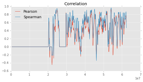
Block-wise Crorrelation

To identify local difference between two maps, block-wise coorelation could be more helpful. A block is created and slided along the diagonal, and for each new position, correlation is calculated.

# Pearson correlation
pearson, p_centers = cmstats.correlateCMaps(ccmapOne, ccmapTwo, diagonal_offset=2, blockSize='1mb',
                                             slideStepSize=1, outFile='pearson.txt', workDir=os.getcwd())


# Spearman correlation
spearman, s_centers = cmstats.correlateCMaps(ccmapOne, ccmapTwo, corrType='spearman', diagonal_offset=2,
                                                 blockSize='1mb', slideStepSize=1, outFile='spearman.txt',
                                                 workDir=os.getcwd())

INFO:correlateCMaps: Block-wise correlation with [1mb] block-size
INFO:correlateCMaps: Number of Blocks: 63
INFO:correlateCMaps: Size of each Block in bins: 10
INFO:correlateCMaps: Number of Overlapping bins between sliding blocks:  9
INFO:correlateCMaps: Block-wise correlation with [1mb] block-size
INFO:correlateCMaps: Number of Blocks: 63
INFO:correlateCMaps: Size of each Block in bins: 10
INFO:correlateCMaps: Number of Overlapping bins between sliding blocks:  9

# Plot the values for visual representations
fig = plt.figure(figsize=(8,4))                               # Figure size

ax = fig.add_subplot(1,1,1)                                   # Axes first plot
ax.set_title('Correlation')                                   # Title first plot

ax.plot(p_centers, pearson, label='Pearson')                  # Plot for Pearson correlation
ax.plot(s_centers, spearman, label='Spearman')                # Plot for Spearman correlation

ax.get_xaxis().get_major_formatter().set_useOffset(False)     # Prevent ticks auto-formatting

plt.legend(loc=2)

plt.show()

path='/home/rajendra/workspace/genome_3d_organization/GM12878_CellLine/HiCmapDataPyObject/resolution_10kb/'
ccmapsOne, ccmapsTwo = [], []
for i in range(1, 23):
    ccmapsOne.append(path+'Chr{0}_NormKR.hicmap'.format(i))
for i in range(1, 23):
    ccmapsTwo.append(path+'Chr{0}_Rawobserved.hicmap'.format(i))

for i in range(len(ccmapsOne)):
    ccmapOne = cmp.load_ccmap(ccmapsOne[i], workDir=os.getcwd())
    ccmapOne.make_readable()

    ccmapTwo = cmp.load_ccmap(ccmapsTwo[i], workDir=os.getcwd())
    ccmapTwo.make_readable()

    print(cmstats.correlateCMaps(ccmapOne, ccmapTwo, corrType='spearman', diagonal_offset=5))
    del ccmapOne
    del ccmapTwo

(0.74487690967318498, 0.0)
(0.74063722421215261, 0.0)
(0.75637101395441264, 0.0)
(0.75799064378987224, 0.0)
(0.76385777207989702, 0.0)
(0.7581134503870115, 0.0)
(0.77085117905282485, 0.0)
(0.78712169997619941, 0.0)
(0.75681100168481319, 0.0)
(0.79607602070672256, 0.0)
(0.79340494862540256, 0.0)
(0.79611875779812202, 0.0)
(0.78246725829489128, 0.0)
(0.81078979072455271, 0.0)
(0.82796003802636897, 0.0)
(0.81646908774859528, 0.0)
(0.8513992946693909, 0.0)
(0.83321467022045526, 0.0)
(0.89497615144311282, 0.0)
(0.89713225129243968, 0.0)
(0.86860067840860633, 0.0)
(0.87945995663009324, 0.0)